Free-Floating Rigid Body Dynamics

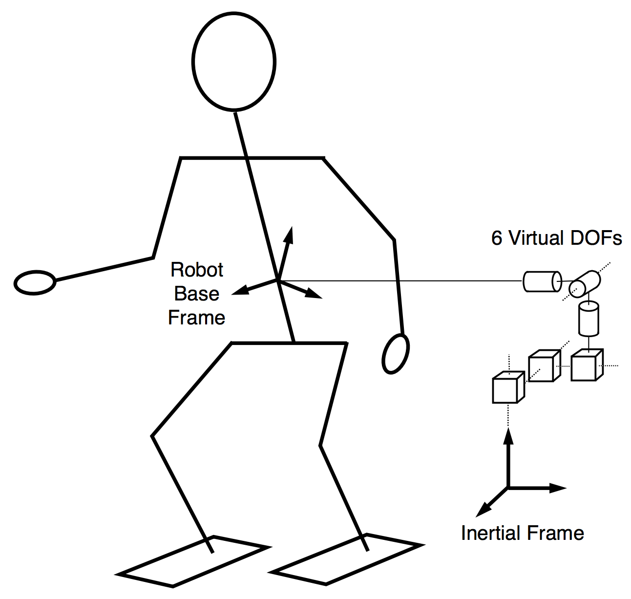
For robots whose root link can float freely in Cartesian space, e.g. humanoids, it is necessary to consider the pose of the root link with respect to (wrt) the inertial reference frame. The primary method for doing so is to account for the root link pose directly in the generalized coordinates, $\q$ , of the robot as shown by:

Todo

add citations

The generalized configuration parameterization for floating base robots,

(1) $\q = \begin{Bmatrix} \gtc_{fb} \\ \q_{j} \end{Bmatrix} \tc$

therefore contains the pose of the base link wrtthe inertial reference frame, $\gtc_{fb}$ , and the joint space coordinates, $\q_j$ . Set brackets are used in (1) because $\gtc_{fb}$ is a homogeneous transformation matrix in $\R^{4\times4}$ and $\q_j$ is a vector in $\R^{n}$ , with $n$ the number of dofof the robot, thus $\gtc_{fb}$ and $\q_{j}$ cannot be concatenated into a vector. However, the twist of the base, $\bs{v}_{fb}$ , with the joint velocities, $\qd_{j}$ , can be concatenated in vector notation, along with the base and joint accelerations to obtain,

(2) $\jsr = \begin{bmatrix} \bs{v}_{fb} \\ \qd_{j} \end{bmatrix} \tc \quad \text{and} \quad \jsrd = \begin{bmatrix} \dot{\bs{v}}_{fb} \\ \qdd_{j} \end{bmatrix} \tp$

These representations provide a complete description of the robot’s state and its rate of change, and allow the equations of motion to be written as,

(3) $M(\q)\jsrd + \underbrace{C(\q, \jsr)\jsr + \bs{g}(\q)}_{\bs{n}(\q, \jsr)} = S^{\top}\torque + \Je^{\top}(\q)\we \tp$

In (3), $M(\q)$ is the generalized mass matrix, $C(\q, \jsr)\jsr$ and $\bs{g}(\q)$ are the Coriolis-centrifugal and gravitational terms, $S$ is a selection matrix indicating the actuated degrees of freedom, $\we$ is the concatenation of the external contact wrenches, and $\Je$ their concatenated Jacobians.

Grouping $C(\q, \jsr)\jsr$ and $\bs{g}(\q)$ together into $\bs{n}(\q, \jsr)$ , the equations can by simplified to

(4) $M(\q)\jsrd + \bs{n}(\q, \jsr) = S^{\top}\torque + \Je^{\top}(\q)\we \tp$

The joint torques induced by friction force could also be included in (4), but are left out for the sake of simplicity. Additionally, the variables $\jsrd$ , $\tau$ , and $\we$ , can be grouped into the same vector,

(5) $\optvar = \bmat{\jsrd \\ \torque \\ \we} \tc$

forming the optimization variable from (1), and allowing (4) to be rewritten as,

(6) $\bmat{-M(\q) & S^{\top} & \Je^{\top}(\q)}\optvar = \bs{n}(\q, \jsr) \tp$

Equation (6) provides an equality constraint which can be used to ensure that the minimization of the control objectives respects the system dynamics.